06. 자연어처리 - 워드 임베딩

1. 워드 임배딩(Word Embedding)

• 단어를 컴퓨터가 이해하고, 효율적으로 처리할 수 있도록 단어를 백터화하는 기술
• 단어를 밀집 백터의 형태로 표현하는 방법
• 워드 임배딩 과정을 통해 나온 결과를 임배딩 백터
• 워드 임배딩을 거쳐 잘 표현된 단어 백터들은 계산이 가능하여, 모델에 입력으로 사용할 수 있음 

 

1. 희소 표현(Sparse Representation)

원 핫 인코딩을 통해서 나온 백터들은 표현하고자 하는 단어의 인덱스의 값만 1이고, 나머지 인덱스에는 전부 0으로 표현되는 백터 표현 방법 원-핫 인코딩에 의해 만들어지는 백터를 '희소 백터'하고 함

2. 희소 백터의 문제점

희소 백터의 특징은 단어의 개수가 늘어나면 백터의 차원이 한없이 커진다는 것 원-핫 백터는 백터 표현 방식이 단순하여, 단순히 단어의 출현 여부만을 백터에 표시할 수 있음 희소 백터를 이용하여 문장 혹은 텍스트 간 유사도를 계산해보면 원하는 유사도를 얻기 힘듬

3. 밀집 표현(Dense Representation)

백터의 차원이 조밀해졌다는 의미 사용자가 설정한 값으로 모든 단어의 백터 표현의 차원을 맞추는 방식 자연어를 밀집 표현으로 변환하는 인코딩 과정에서 0과 1의 binary값이 아니라, 연속적인 실수 값을 가질 수 있음 적은 차원으로 대상을 표현할 수  있음 더 큰 일반화 능력을 가지고 있음

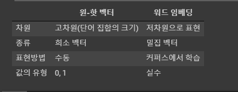
4. 원-핫 백터와 워드 임배딩의 차이

원 핫 백터: 고차원, 희소 백터, 값의 유형이 0과 1 워드 임베딩: 저차원, 밀집 백터, 실수

5. 차원 축소(Dimensionality Reduction)

희소 백터를 밀집 백터의 형태로 변환하는 방법 머신러닝에서는 많은 피처들로 구성된 고차원의 데이터에서 중요한 피처만 뽑아 저차원의 데이터(행, 렬)로 변환하기 위해 사용 PCA(Principal Component Analysis), 잠재 의미 분석(Latent Semantic Analysis), 잠재 디리클레할당(Latent Dirichlet Allocation), SVD(Singular Value Decomposition)

 

 

 

 

2. 주요 워드 임베딩 알고리즘

• 워드 임베딩은 고차원 단어 공간에서 저차원의 벡터 공간으로 변환하는 방법
• 변환된 백터는 단어의 유사성을 반영하며, 유사한 의미를 가진 단어들은 백터 공간에 가깝게 위치
• 모델이 텍스트 데이터의 의미를 이해하고 학습할 수 있도록 함

 

1. Word2Vec

분포 가설 하에 표현한 분산 표현을 따르는 워드 임베딩 모델  분산 표현(Distributed Representation) 분포 가설: 비슷한 문맥에서 등장하는 단어들을 비슷한 의미를 가진다는 가설 분포 가설의 목표는 단어 주변의 단어들, window 크기에 따라 정의되는 문맥의 의미를 이용해 단어를 백터로 표현(분산 표현)하는 것 분산 표현으로 표현된 백터들은 원-핫 백터처럼 차원이 단어 집합의 크기일 필요가 없으므로, 백터의 차원이 상대적으로 저차원으로 줄어듬 희소 표현에서는 각각의 차원이 각각의 독립적인 정보를 가지고 있지만,  밀집에서는 하나의 차원이 여러 속성들이 버무려진 정보를 갖고 있음  밀집 표현을 분산 표현이라 부르기도 함, 밀집 표현을 이용한 대표적인 학습 방법이 Word2Vec 임  중심 단어와 주변의 단어들을 사용하여 단어를 예측하는 방식으로 임베딩을 만듦 Google이 2013년도 처음 공개한 모델 Word2Vec의 학습 방식에는 CBOM(Continuous Bag od Words), Skip-Gram을 사용  CBOW(Continuous Bag of Words) 주변에 있는 단어들을 보고 중간에 있는 단어를 예측하는 방법 주변 단어(context)는 타겟 단어(targer word)의 직전 n개 단어와 직후 n개 단어를 의미하며, 이 범위를 window라 부르고, n을 window size라고 부름 문장 하나에 대해 한 번만 학습을 진행하는 것은 가깝기 때문에 sliding window방식을 사용하여 하나의 문장을 가지고 여러개의 학습 데이터셋을 만듦 Skip-gram 중심 단어에서 주변 단어를 예측 중심 단어를 sliding window 하면서 학습 데이터를 증강 중심 단어를 가지고 주변 단어를 예측하는 방법이기 때문에 projection layer에서 백터들 간의 평균을 구하는 과정이 없으며, 대신 output layer를 통해 백터가 window size의 2n개 만큼 나옴 CBOW 와 Skip-gram의 차이점  Skip-gram이 CBOW에 비해 문맥을 고려하기 때문에 Skip-gram의 성능이 일반적으로 더 좋음 Skip-gram이 단어 당 학습 횟수가 더 많고, 임베딩의 조정 기회가 많으므로 더 정교한 임배딜 학습이 가능  Word2Vec의 한계점 단어의 형태학적 특성을 반영하지 못함 예) teach, teacher, teachers 와 같은 3단어는 의미적으로 유사한 단어지만 각 단어를 개별단어로 처리하여 3단어 모두 백터 값이 다르게 구성됨 단어 빈도 수의 영향을 많이 받아 희소한 단어를 임배딩하기 어려움  OOV(Out of Vocabulary)의 처리가 어려움 새로운 단어가 등장하면 데이터 전체를 다시 학습시켜야 함  단어 사전의 크기가 클수록 학습하는데 오래걸림

2. FastText

2017년 페이스북 AI Reserarch 팀에서 개발한 텍스트 분류 및 단어 벡터 표현 도구 대규모 데이터셋에서 빠르게 작동하도록 설계, 단어 임베딩과 텍스트 분류 모두에 사용할 수 있음 동작 원리  <, >는 단어의 경계를 나타나기 위한 특수 기호  단어를 먼저 <, >로 감싼 후 설정한 n-gram의 값에 따라 앞에서 부터 단어를 쪼갬 예) "apple" ["a","ap"."app","appl","apple","p","pp", "ppl"."ple","e"] 마지막에 본 단어르 설명하기 위해 <, >으로 감싸진 전체 단어를 하나 추가함 장점 오타나 모르는 단어에 대한 대응이 쉽다 단어 집합 내 빈도 수가 적었던 단어에 대한 대응 자연어 토퍼스 내 노이즈에 대응

 

3. 워드 임베딩 구축하기

 

◼  import

import pandas as pd         import numpy as np         from sklearn.datasets import fetch_20newsgroups

 

 

◼ 데이터 셋 - fetch_20newsgroups

dataset = fetch_20newsgroups(shuffle = True, random_state = 2024, remove = ('headers', 'footers', 'quotes'))         dataset = dataset.data         dataset

['Hell, just set up a spark jammer, or some other _very_ electrically-noisy\ndevice. Or build an active Farrady cage around the room, with a "noise"\nsignal piped into it. While these measures will not totally mask the\nemissions of your equipment, they will provide sufficient interference to\nmake remote monitoring a chancy proposition, at best. There is, of course,\nthe consideration that these measures may (and almost cretainly will)\ncause a certain amount of interference in your own systems. It\'s a matter\nof balancing security versus convenience.\n\nBTW, I\'m an ex-Air Force Telecommunications Systems Control Supervisor and\nTelecommun .......  '\n\n\n\n    The joystick reads in anolog values through a digital port. How?\n    You send a command to the port to read it, then you time how long\n    it takes for the joystick port to set a certain bit.  This time\n    is proportional to the joystick position.  Obviously, since time\n    is used as a position, you cannot get rid of this ridiculus waste \n    of time.  If you wrote your own routine instead of the BIOS, it\n    would speed it up some, but the time would still be there.\n\n-- ',  '88 toyota Camry - Top Of The Line Vehicle\nblue book $10,500\nasking 9,900.\n\n73 k miles\nauto transmission\n \nHas Everything!\n\nowned by a meticulous automoble mechanic\n\ncall (408) 425-8203 ask for Bob.',

 

 

 

◼ 첫번째 항목 , 데이터셋 길이 출력 

dataset[0]         len(dataset)

Hell, just set up a spark jammer, or some other _very_ electrically-noisy\ndevice. Or build an active Farrady cage around the room, with a "noise"\nsignal piped into it. While these measures will not totally mask the\nemissions of your equipment, they will provide sufficient interference to\nmake remote monitoring a chancy proposition, at best. There is, of course,\nthe consideration that these measures may (and almost cretainly will)\ncause a certain amount of interference in your own systems. It\'s a matter\nof balancing security versus convenience.\n\nBTW, I\'m an ex-Air Force Telecommunications Systems Control Supervisor and\nTelecommunications/Cryptographic Equipment Technician.\n ----------------------------------------------------------------------------------------------------------------------------- 11314

 

 

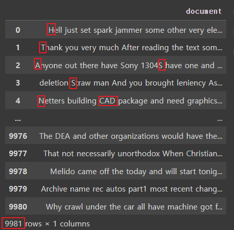
◼ 컬럼명을 document로 한 데이터프레임으로 변환

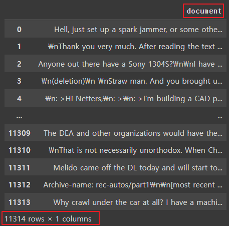
news_df = pd.DataFrame({'document': dataset})         news_df

 

 

 

◼ 데이터 셋의 결측치 제거

# 데이터 셋의 결측치 제거         news_df = news_df.dropna().reset_index(drop = True)         print(f'필터링된 데이터의 총 개수: {len(news_df)}')

필터링된 데이터의 총 개수: 11314  -------------------------------------------------- (결측치없음)

 

 

◼ 열기준으로 중복된 데이터를 제거

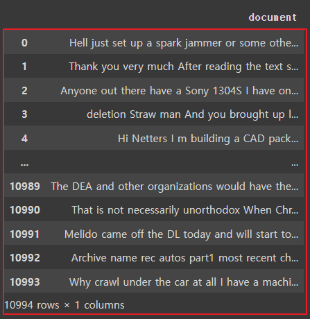
# 열 기준으로 중복된 데이터를 제거         processed_news_df = news_df.drop_duplicates(['document']).reset_index(drop = True)         print(f'필터링된 데이터의 총 개수: {len(processed_news_df)}')

필터링된 데이터의 총 개수: 10994 -------------------------------------------------- 중복데이터 320개 삭제

 

 

◼ 데이터 중 특수 문자 제거

# 데이터 중 특수 문자 제거         processed_news_df['document'] = processed_news_df['document'].str.replace('[^a-zA-Z0-9]', ' ', regex=True)         processed_news_df

특수문자들이 삭제된 것을 볼 수 있음

 

 

◼  데이터셋의 길이가 너무 짧은 단어(길이가 2 이하)를 제거

# 데이터셋의 길이가 너무 짧은 단어를 제거(단어 길이가 2 이하)         processed_news_df['document'] = processed_news_df['document'].apply(lambda x: ' '.join([token for token in x.split() if len(token) > 2]))         processed_news_df

단어길이가 짧은 것이 삭제되었음

 

 

◼ 전체 문장이 100자 이상, 단어의 길이가 3개 이상인 데이터를 필터링 

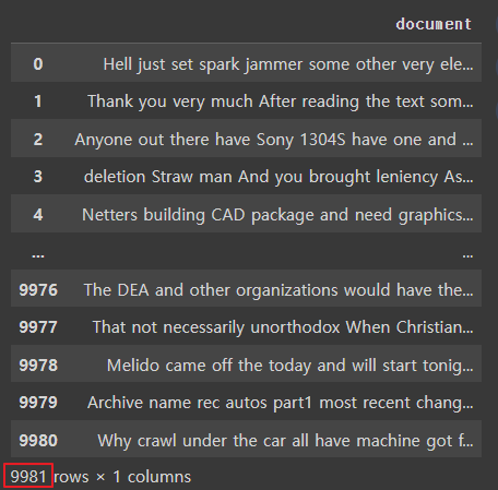
# 전체 문장이 100자 이상이거나 단어의 길이가 3개 이상인 데이터를 필터링           processed_news_df = processed_news_df[processed_news_df.document.apply(lambda x: len(str(x)) >= 100 and len(str(x).split()) >= 3)].reset_index(drop=True)           processed_news_df

 

 

◼  전체 단어에 대해 소문자로 변환 

# 전체 단어에 대해 소문자로 변환           processed_news_df['document'] = processed_news_df['document'].apply(lambda x: x.lower())           processed_news_df

대문자가 다 소문자로 바뀜

 

 

 

◼ 데이터셋에 불용어를 제거하기

• 영어 불용어 개수 확인

# 데이터셋에 불용어를 제외하기 위해 확인         import nltk         from nltk.corpus import stopwords         nltk.download('stopwords')         stop_words = stopwords.words('english')         print(len(stop_words))

179

 

• 불용어를 제외하고, 띄어쓰기 단위로 문장을 분리하여 리스트로 저장

# 데이터셋에서 불용어를 제외하고, 띄어쓰기 단위로 문장을 분리하여 리스트로 저장         tokenized_doc = processed_news_df['document'].apply(lambda x: x.split())         tokenized_doc = tokenized_doc.apply(lambda x: [s_word for s_word in x if s_word not in stop_words])         tokenized_doc

 

 

◼ 토큰화

from tensorflow.keras.preprocessing.text import Tokenizer         tokenizer = Tokenizer()         tokenizer.fit_on_texts(tokenized_doc)         word2idx = tokenizer.word_index         print(word2idx)         idx2word = {value: key for key, value in word2idx.items()}         print(idx2word)

{'one': 1, 'would': 2, 'max': 3, 'people': 4, 'like': 5, 'get': 6, 'know': 7, 'also': 8, 'use': 9, 'think': 10, 'time': 11, 'new': 12, 'could': 13, 'well': 14, 'good': 15, 'may': 16, 'edu': 17, 'even': 18, 'two': 19, 'first': 20, 'see': 21, 'many': 22, 'much': 23, 'way': 24, 'make': 25, 'system': 26, 'god': 27, 'used': 28, 'say': 29, 'right': 30, 'file': 31, 'said': 32, 'want': 33, 'need': 34, 'work': 35, 'anyone': 36, 'something': 37,....'webers': 97000, 'overgeneralization': 97001, '455cid': 97002, 'cabot': 97003, 'decant': 97004} ------------------------------------------------------------------------------------------------------------------------------------ {1: 'one', 2: 'would', 3: 'max', 4: 'people', 5: 'like', 6: 'get', 7: 'know', 8: 'also', 9: 'use', 10: 'think', 11: 'time', 12: 'new', 13: 'could', 14: 'well', 15: 'good', 16: 'may', 17: 'edu', 18: 'even', 19: 'two', 20: 'first', 21: 'see', 22: 'many', 23: 'much', 24: 'way', 25: 'make', 26: 'system', 27: 'god', 28: 'used', 29: 'say', 30: 'right', 31: 'file', 32: 'said', 33: 'want', 34: 'need', 35: 'work', 36: 'anyone', 37: 'something' .... 97000: 'webers', 97001: 'overgeneralization', 97002: '455cid', 97003: 'cabot', 97004: 'decant'}

 

 

◼ encoded: 각 문장을 정수 인덱스 시퀀스로 변환

encoded = tokenizer.texts_to_sequences(tokenized_doc)         encoded

[[526,   96,   8720,   20921,   20922,   7462,   633,   417 .....   412,   88,   15,   4,   1059,   2818,   803,   130,   412],  ...]

 

 

◼ 단어 사전의 크기 확인

# 단어 사전 크기 확인         vocab_size = len(word2idx)         print(f'단어 사전의 크기: {vocab_size}')

단어 사전의 크기: 97004

 

 

◼ Word2Vec 알고리즘에서 단어 벡터를 학습
: 스킵그램 모델을 적용해 단어 쌍을 생성

# 텍스트 데이터를 다루는 과정에서 단어 쌍을 생성하는 데 사용           # Skip-gram 모델을 사용하여 단어 쌍을 만들며, Word2Vec 알고리즘의 구성요소           # 주어진 단어를 기준으로 주변 단어를 예측하는 방식으로 단어 벡터를 학습           from tensorflow.keras.preprocessing.sequence import skipgrams           # 샘플 만들기           # skip_grams(시퀀스, 사전크기, 윈도우크기)           # 시퀀스 : 인코딩한 리스트           # 사전크기: 단어 사전의 크기, 시퀀스에 등장하는 단어의 총 개수           # 중심단어와 주변단어간의 최대거리           skip_grams = [skipgrams(sample, vocabulary_size = vocab_size, window_size = 10) for sample in encoded[:5]]           print(f'전체 샘플 수: {len(skip_grams)}')           print(f'첫번째 샘플의 크기: {len(skip_grams[0])}')           print(f'첫번째 샘플: {skip_grams[0]}')

전체 샘플 수: 5 첫번째 샘플의 크기: 2 첫번째 샘플: ([[422, 64712], [2807, 30446], [336, 1245], [344, 24409], [315, 2170] ....0, 0, 0, 0, 1, 1, 1, 1, 1, 1, 1, 1, 0, 1, 1, 1, 1, 0, 1, 1, 1, 1, 1, 1

 

 

 

◼ 스킵그램 모델을 사용하여 생성된 단어 쌍과 해당 레이블을 출력

# pairs: (중심단어, 주변단어) 형태의 단어 쌍 리스트       # labels : 각 단어 쌍의 레이블 리스트로, 해당 단어 쌍이 실제로 등장하는지 여부를 나타냄       pairs, labels = skip_grams[0][0], skip_grams[0][1]       print(pairs)       print(labels)

[[422, 64712], [2807, 30446], [336, 1245], [344, 24409], [315, 2170], [109, 13326] [0, 1, 1, 0, 1, 0, 1, 1, 1, 1, 1, 0, 1, 1, 0, 1, 0, 1, 0, 1, 1, 1, 1, 1, 1, 0

부정적 예: 중심 단어와 실제 텍스트에서 함께 등장하지 않은 단어 쌍. 이러한 경우 레이블은 0입니다. 긍정적 예: 중심 단어와 실제 텍스트에서 함께 등장한 주변 단어 쌍. 이러한 경우 레이블은 1입니다.

 

 

◼ 단어 쌍의 개수와
각 단어 쌍에 대한 레이블의 개수 확인

print(len(pairs))         print(len(labels))

2060 2060

 

 

◼ idx2word 딕셔너리: 중심 단어와 주변 단어의 인덱스쌍

for i in range(5):               print('({:s}({:d}), {:s}({:d})) -> {:d}'.format(                   idx2word[pairs[i][0]], pairs[i][0],                   idx2word[pairs[i][1]], pairs[i][1],                   labels[i]               ))

(force(422), trifercation(64712)) -> 0 (measures(2807), piped(30446)) -> 1 (almost(336), remote(1245)) -> 1 (provide(344), ctrller(24409)) -> 0 (matter(315), consideration(2170)) -> 1

idx2word[pairs[i][0]]와 idx2word[pairs[i][1]]는 각각 pairs[i]에서 첫 번째와 두 번째 요소의 인덱스를 실제 단어로 변환합니다. pairs[i][0]와 pairs[i][1]은 각각 중심 단어와 주변 단어의 인덱스를 나타냅니다. labels[i]는 각 단어 쌍의 레이블을 나타내며, 1은 긍정적 예(실제 등장한 경우), 0은 부정적 예(실제 등장하지 않은 경우)를 의미합니다.

 

 

◼ 인코딩된 문서(encoded)의 처음 9981개를 사용
스킵그램 데이터셋(training_dataset)을 생성,  데이터셋의 길이를 확인

training_dataset = [skipgrams(sample, vocabulary_size = vocab_size, window_size = 10) for sample in encoded[:9981]]           len(training_dataset)

9981

 

 

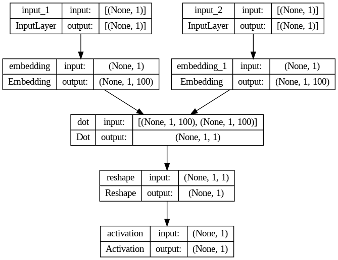
◼ 중심 단어를 위한 임베딩 테이블

from tensorflow.keras.models import Sequential, Model       from tensorflow.keras.layers import Embedding, Reshape, Activation, Input, Dot       from tensorflow.keras.utils import plot_model       # 단어 임베딩의 차원을 100으로 설정       embeding_dim = 100       # 신경망의 입력 레이어를 생성합니다.       # 모양은 (1,)으로 설정되어 있어 단일 정수 값을 입력으로 받습니다           (일반적으로 어휘 사전에서 단어의 인덱스를 나타냅니다).       w_inputs = Input(shape = (1,), dtype = 'int32')       # 임베딩 레이어를 생성합니다       # 입력 레이어 (w_inputs)에서 제공된 정수 인덱스를 가져와 이를 고정 크기의 밀집 벡터로 변환       word_enbedding = Embedding(vocab_size, embeding_dim)(w_inputs)       c_inputs = Input(shape = (1,), dtype = 'int32')       context_enbedding = Embedding(vocab_size, embeding_dim)(c_inputs)       dot_product = Dot(axes = 2)([word_enbedding, context_enbedding])       dot_product = Reshape((1,), input_shape = (1,1))(dot_product)       output = Activation('sigmoid')(dot_product)       model = Model(inputs = [w_inputs, c_inputs], outputs = output)       model.summary()

 

 

 

◼  모델 등록 후 시각화

# 모델 시각화         model.compile(loss = 'binary_crossentropy', optimizer = 'adam')         plot_model(model, to_file = 'model.png', show_shapes = True, show_layer_names = True)

 

 

 

◼ 모델 학습

# 모델 학습         for epoch in range(100):           loss = 0           for _, elem in enumerate (skip_grams):             first_elem = np.array(list(zip(*elem[0]))[0], dtype = 'int32')             second_elem = np.array(list(zip(*elem[0]))[1], dtype = 'int32')             labels = np.array(elem[1], dtype = 'int32')             X = [first_elem, second_elem]             y = labels             loss += model.train_on_batch(X, y)           print('Epoch: ', epoch + 1, 'Loss: ',loss)

 

 

◼ 

# WOrd2Vec 모델을 학습시키고 학습된 모델을 활용하여 단어간 유사도 측정         # Gansim         # 자연어처리작어베서 주로 사용되는 오픈 소스 라이브러리         # 토픽 모델링, 문서유사도 계산, 단어 임베딩(Word2Bec,FastText)         import gensim         vectors = model.get_weights()[0]         len(vectors)

97004

 

 

 

◼ 파일로 저장

f = open('vectors.txt', 'w')         f.write('{} {}\n'.format(vocab_size, embeding_dim))         for word ,i in tokenizer.word_index.items():             f.write('{} {} \n'.format(word, ' '.join(map(str, list(vectors[i-1, :])))))         f.close()

 

 

◼ 유사한 단어 확인 

# 유사한 단어 확인         w2v = gensim.models.KeyedVectors.load_word2vec_format('./vectors.txt', binary=False)         w2v.most_similar(positive = ['doctor'])         w2v.most_similar(positive = ['apple'])

[('driver', 0.9293440580368042),  ('possible', 0.9281030893325806),  ('break', 0.9268569946289062),  ('say', 0.925711452960968),  ('mean', 0.9256541132926941),  ('like', 0.9255044460296631),  ('government', 0.9252896308898926),  ('religious', 0.9251723885536194),  ('users', 0.9251695871353149),  ('b8f', 0.9251244068145752)] ---------------------------------------------------- [('vers', 0.9807016253471375),  ('teaches', 0.9797495007514954),  ('separate', 0.979489803314209),  ('wow', 0.979457437992096),  ('randomizer', 0.9793667197227478),  ('novice', 0.9793640971183777),  ('historical', 0.9789345860481262),  ('duty', 0.9788818955421448),  ('ability', 0.978827178478241),  ('closely', 0.9788203239440918)]