1. 인사자료 데이터셋
- 작업파일
- import
import numpy as np
import pandas as pd
import seaborn as sns
import matplotlib.pyplot as plt
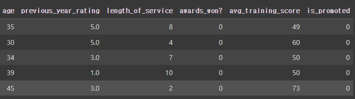
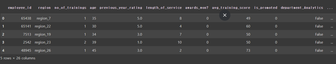
- 데이터 가져오기
hr_df=pd.read_csv('/content/drive/MyDrive/1. KDT/6. 머신러닝 딥러닝/데이터/hr.csv')
hr_df.head()
 |
 |
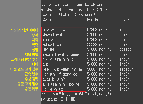
- 정보보기
hr_df.info()
 |
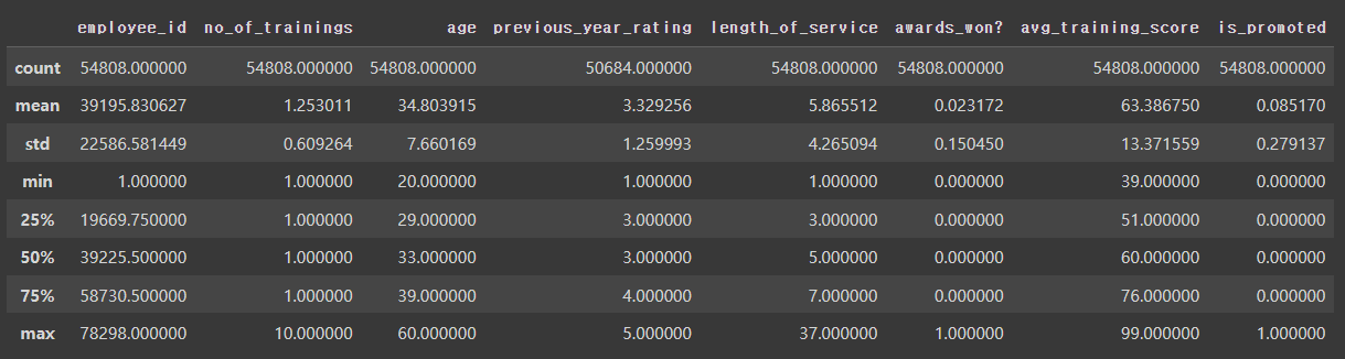
- 통계치보기
hr_df.describe()
 |
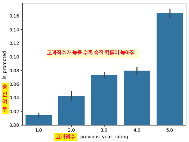
- 고과점수에 따른 승진여부 그래프로 보기
sns.barplot(x= 'previous_year_rating',y='is_promoted',data=hr_df)
 |
- lineplot 그래프로 보기
sns.lineplot(x= 'previous_year_rating',y='is_promoted',data=hr_df)
 |
- 고과점수에 따른 승진여부 그래프로 보기
sns.lineplot(x= 'avg_training_score',y='is_promoted',data=hr_df)
 |
- 채용방법에 따른 승진여부
sns.barplot(x= 'recruitment_channel',y='is_promoted',data=hr_df)
hr_df['recruitment_channel'].value_counts()
  |
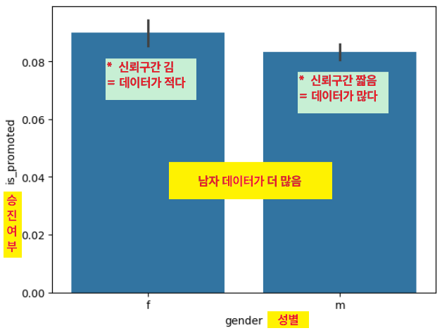
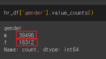
- 성별에 따른 승진여부
sns.barplot(x= 'gender',y='is_promoted',data=hr_df)
hr_df['gender'].value_counts()
 |
 |
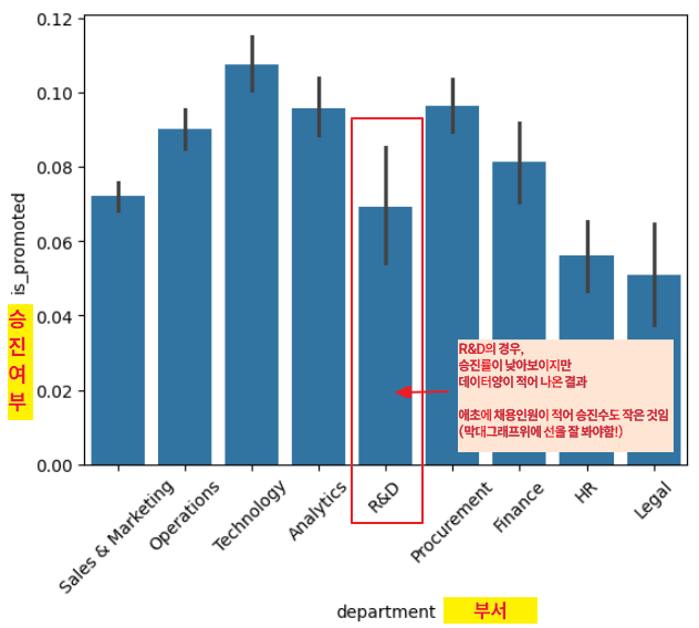
- 부서별 승진여부
sns.barplot(x= 'department',y='is_promoted',data=hr_df)
plt.xticks(rotation=45) # 글씨가 길어 겹칠때 이용
hr_df['department'].value_counts()
  |
- 지역에 따른 승진여부
plt.figure(figsize=(14,10))
sns.barplot(x='region',y='is_promoted',data=hr_df)
plt.xticks(rotation=45)
 |
- null 인 데이터 확인
hr_df.isna().mean()
 |
- null인 열 살펴보기
중요한 정보가 아닌 것 같음!
hr_df['education'].value_counts()
hr_df['previous_year_rating'].value_counts()
  |
- education, previous_year_rating 열 날리기
hr_df = hr_df.dropna()
hr_df.info()
 |
- 각 열의 고유한 값의 개수
for i in ['department','region','education','gender','recruitment_channel']:
print(i,hr_df[i].nunique())
 |
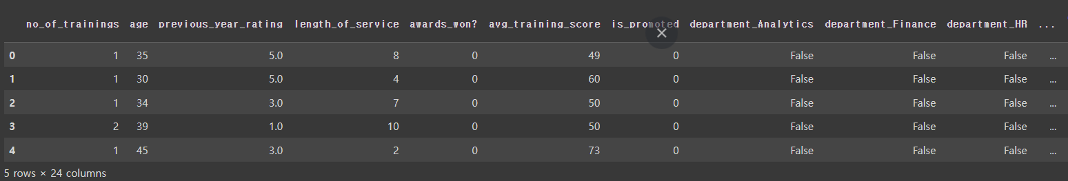
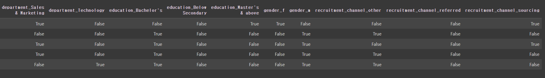
- 'department','education','gender','recruitment_channel' 원인핫인코딩
hr_df = pd.get_dummies(hr_df, columns=['department','education','gender','recruitment_channel'])
hr_df.head()
  |
- 필요없는 행 'employee_id','region' 날리기
hr_df.drop(['employee_id','region'],axis=1, inplace=True)
hr_df.head()
  |
- 데이터 나누기
from sklearn.model_selection import train_test_split
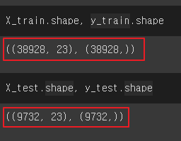
X_train,X_test,y_train,y_test = train_test_split(hr_df.drop('is_promoted',axis=1),hr_df['is_promoted'],test_size=0.2,random_state=10)
X_train.shape, y_train.shape
X_test.shape, y_test.shape
 |
2. 로지스틱 회귀(Logistic Regression)
로지스틱 회귀(Logistic Regression)로지스틱 회귀는 두 가지 중 하나를 결정하는 문제(이진 분류)를 해결하기 위한 대표적인 알고리즘입력 데이터와 가중치의 선형 조합을 통해 선형 방정식을 생성하고, 그 결과를 0과 1 사이의 확률값으로 변환 (시그모이드 함수) 주요 특징
다중 클래스 분류 (Multiclass Classification)로지스틱 회귀는 원래 이진 분류를 위해 고안되었지만,몇 가지 확장을 통해 다중 클래스 분류 문제에도 적용할 수 있습니다. 다중 클래스 분류를 위해 두 가지 주요 전략을 사용합니다:
선호도
정리로지스틱 회귀는 이진 분류 문제를 해결하기 위한 알고리즘으로,입력 데이터와 가중치의 선형 조합을 시그모이드 함수를 통해 0과 1 사이의 확률값으로 변환합니다. 다중 클래스 분류의 경우 OvR과 OvO 전략을 사용하여 확장할 수 있으며, 대부분 OvR 전략이 선호되지만, 데이터의 불균형이 심한 경우 OvO 전략이 더 효과적일 수 있습니다. |
- 학습시키기
from sklearn. linear_model import LogisticRegression
lr=LogisticRegression()
lr.fit(X_train ,y_train)
 |
- 로지스틱 회귀 모델을 사용하여
테스트 데이터에 대한 예측을 수행
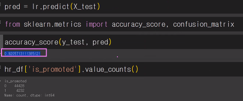
pred = lr.predict(X_test)
- 모델의 예측 성능을 평가
: accuracy_score는 실제 레이블과 예측된 레이블을 비교하여 정확도를 계산
from sklearn.metrics import accuracy_score
accuracy_score(y_test,pred)
| 0.9201602959309494 * 로지스틱 회귀이기 때문에 정확도를 의심할 필요가 있음 ( 데이터가 쏠려있나?) |
- 'is_promoted' 열의 값 빈도를 계산
hr_df['is_promoted'].value_counts()

|
3. 혼돈 행렬(confusion matrix)
- 정밀도와 재현율( 민감도 )을 활용하여 평가용 지수
- array (TN, FP, FN, TP)
혼돈 행렬 (Confusion Matrix)혼돈 행렬은 실제 클래스와 예측된 클래스 간의 관계를 나타내는 행렬입니다.이 행렬은 분류 문제에서 네 가지 결과를 나타냅니다:
|
- 예측 결과를 바탕으로 혼동 행렬(confusion matrix)을 계산
from sklearn. metrics import accuracy_score,confusion_matrix
confusion_matrix(y_test,pred)
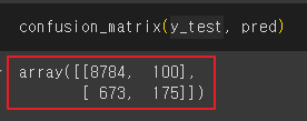 |
| TN(8784) FP(100) FN(673) TP(175) * TN: 승진하지 못했는데, 승진하지 못했다고 예측 * FN: 승진하지 못했는데, 승진했다고 예측 * FP: 승진했는데, 승진하지 못했다고 예측 * TP: 승진했는데, 승진하지 못했다고 예측 |
1. 정밀도(precision) * TP / (TP + FP) * 무조건 양성으로 판단해서 계산하는 방법 * 실제 1이라고 예측한것 중에 얼마 만큼을 제대로 맞췄는가? * 모델이 양성(Positive)으로 예측한 것 중에서 실제로 양성인 비율 2. 재현율(recall) * TP / (TP+FN) * 1이라고 양성인 것 중에서 모델이 양성으로 예측한 비율 * 민감도 또는 TPR(True Positive Rate)라고도 부름 * 실제로 양성인 것 중에서 모델이 양성으로 예측한 비율 3. f1 score * 정밀도와 재현율의 조화평균을 나타내는 지표 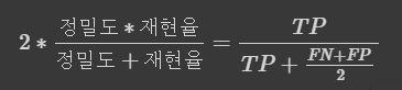 - 산술평균(Arithmetic Average): 값들의 합을 값의 개수로 나눈 것 - 조화평균(Harmonic Average): 값들의 역수들의 산술평균의 역수, 조화평균은 작은 값에 더 많은 가중치를 부여합니다. |
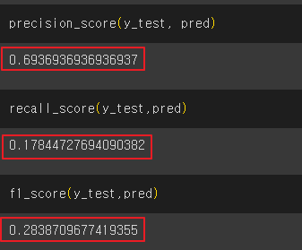
- 분류 모델의 성능을 평가
scikit-learn 라이브러리의 precision_score, recall_score, f1_score 함수를 사용
from sklearn.metrics import precision_score, recall_score, f1_score
precision_score(y_test, pred)
recall_score(y_test,pred)
f1_score(y_test,pred)
 |
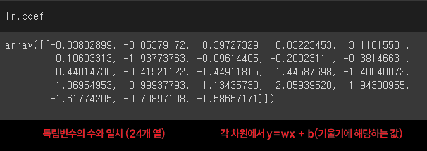
- 회귀 모델에서 각 특성(feature)에 대한 회귀 계수(기울기)
lr.coef_# 24개 컬럼에 대한 기울기
 |
- 로지스틱 회귀 모델을 사용하여 독립변수와 종속변수 간의 관계를 학습
# 영향력 있을 수 있는 독립변수 3개
tempX=hr_df[['previous_year_rating','avg_training_score','awards_won?']]
# 종속변수 1개
tempy = hr_df['is_promoted']
temp_lr =LogisticRegression()
# 학습시키기
temp_lr.fit(tempX,tempy)
 |
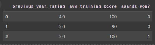
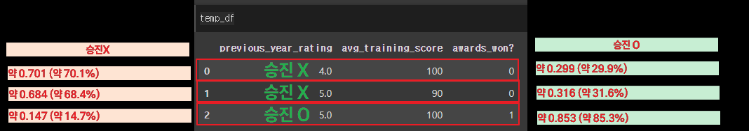
- temp_df 데이터프레임 생성
temp_df = pd.DataFrame({
'previous_year_rating':[4.0, 5.0, 5.0],
'avg_training_score':[100,90,100],
'awards_won?':[0, 0, 1]
})
temp_df
|
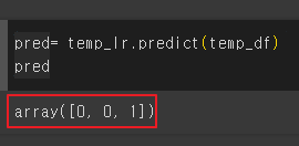
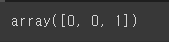
- temp_df에 대해 모델이 예측한 값을 반환
세 명의 직원에 대한 승진 여부 예측 값
해당 직원이 승진했는지(1) 아니면 승진하지 않았는지(0)를 나타내기
pred= temp_lr.predict(temp_df)
pred
 |
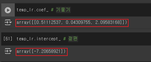
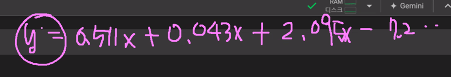
- 모델이 각 특성에 어떤 가중치를 부여하고, 전체적으로 어떤 경계를 설정하는지를 이해
temp_lr.coef_ # 기울기
temp_lr.intercept_ # 절편
|
  |
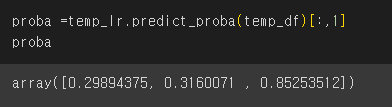
- 테스트 데이터에 대한 예측 확률을 계산
proba =temp_lr.predict_proba(temp_df)
proba
|
- temp_lr 로지스틱 회귀 모델을 사용하여
temp_df 데이터프레임의 각 샘플에 대해 양성 클래스(즉, 승진될 확률)를 예측하는 과정
proba =temp_lr.predict_proba(temp_df)[:,1]
proba
 |
- 임계값을 설정하여 확률 값을 이진 예측으로 변환하는 과정
# 임계값 설정
# 기본 임계값은 0.5
threshold = 0.5
pred = (proba > threshold).astype(int)
pred
 |
4. 교차 검증(Cross Validation)
- train_test_split에서 발생하는 데이터의 섞임에 따라 성능이 좌우되는 문제를 해결하기 위한 기술
- k겹(Fold) 교차 검증을 가장 많이 사용
- import
from sklearn.model_selection import KFold
- KFold 객체 생성
: splits = 5 -> 데이터를 5개로 나눔 (훈련 4 테스트 1)
kf = KFold(n_splits=5)
kf
| KFold(n_splits=5, random_state=None, shuffle=False) |
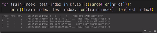
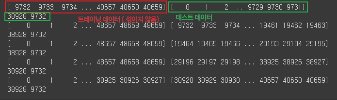
- KFold를 사용하여 데이터를 분할하고 인덱스 출력
for train_index, test_index in kf.split(range(len(hr_df))):
print(train_index, test_index)
print(len(train_index), len(test_index))
 |
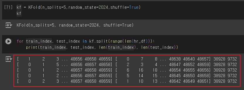
- 섞어서 다시 진행
kf = KFold(n_splits=5,random_state=2024,shuffle=True)
kf
for train_index, test_index in kf.split(range(len(hr_df))):
print(train_index, test_index, len(train_index), len(test_index))

 |
- KFold를 사용하여 데이터를 분할하고 각 폴드에서의 정확도를 측정
# KFold(n=5)를 사용하여 위 데이터를 LogisticRegression 모델로 학습시키고
# 각 n마다 예측결과를 출력
acc_list = []
# KFold를 사용하여 데이터를 분할하고 각 폴드에서의 정확도를 측정
for train_index, test_index in kf.split(range(len(hr_df))):
# 독립변수와 종속변수 설정
X = hr_df.drop('is_promoted', axis=1)
y = hr_df['is_promoted']
# 학습 데이터와 테스트 데이터 생성
X_train = X.iloc[train_index]
X_test = X.iloc[test_index]
y_train = y.iloc[train_index]
y_test = y.iloc[test_index]
# 로지스틱 회귀 모델 학습
lr = LogisticRegression()
lr.fit(X_train, y_train)
# 테스트 데이터에 대한 예측 수행
pred = lr.predict(X_test)
# 정확도를 리스트에 추가
acc_list.append(accuracy_score(y_test, pred))
# 정확도 리스트 출력
print(acc_list)
# 정확도의 평균 계산
np.array(acc_list).mean()
더보기
accuracy 값이 다양하게 나옴
 |
'AI > 머신러닝' 카테고리의 다른 글
| 09. 랜덤 포레스트 (Random Forest) | Hotel (0) | 2024.06.12 |
|---|---|
| 08. SVM, Scaling | 손글씨 (0) | 2024.06.12 |
| 06. 의사결정 나무(Decision Tree) | 자전거 (0) | 2024.06.11 |
| 05. 선형회귀(Linear Regression) | Rent (0) | 2024.06.11 |
| 04. 데이터 전처리 | 타이타닉 (1) | 2024.06.10 |


