09. 랜덤 포레스트 (Random Forest) | Hotel

1. Hotel 데이터셋

  

 

• 파일 가져오기

  

 

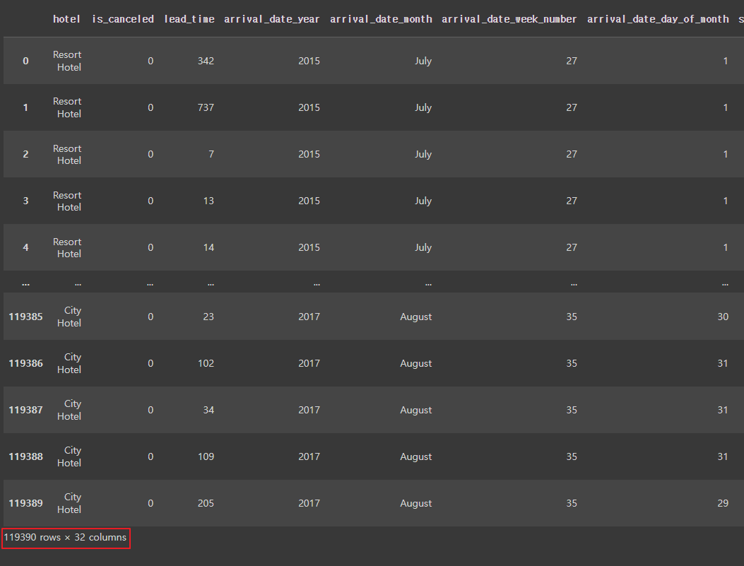
      hotel_df = pd.read_csv('/content/drive/MyDrive/1. KDT/6. 머신러닝 딥러닝/데이터/hotel.csv')

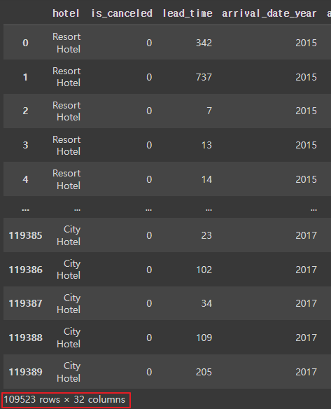
      hotel_df

 

  

 

 

• 정보보기

 

 

        hotel_df.info()

 

  

* hotel: 호텔 종류 * is_canceled: 취소 여부 * lead_time: 예약 시점으로부터 체크인 될 때까지의 기간(얼마나 미리 예약했는지) * arrival_date_year: 예약 연도 * arrival_date_month: 예약 월 * arrival_date_week_number: 예약 주 * arrival_date_day_of_month: 예약 일 * stays_in_weekend_nights: 주말을 끼고 얼마나 묶었는지 * stays_in_week_nights: 평일을 끼고 얼마나 묶었는지 * adults: 성인 인원수 * children: 어린이 인원수 * babies: 아기 인원수 * meal: 식사 형태 * country: 지역 * distribution_channel: 어떤 방식으로 예약했는지 * is_repeated_guest: 예약한적이 있는 고객인지 * previous_cancellations: 몇번 예약을 취소했었는지 * previous_bookings_not_canceled: 예약을 취소하지 않고 정상 숙박한 횟수 * reserved_room_type: 희망한 룸타입 * assigned_room_type: 실제 배정된 룸타입 * booking_changes: 예약 후 서비스가 몇번 변경되었는지 * deposit_type: 요금 납부 방식 * days_in_waiting_list: 예약을 위해 기다린 날짜 * customer_type: 고객 타입 * adr: 특정일에 높아지거나 낮아지는 가격 * required_car_parking_spaces: 주차공간을 요구했는지 * total_of_special_requests: 특별한 별도의 요청사항이 있는지 * reservation_status_date: 예약한 날짜 * name: 이름 * email: 이메일 * phone-number: 전화번호 * credit_card: 카드번호

 

 

• 필요없는 데이터 삭제

  

 

          # 필요없는 데이터 삭제

          hotel_df.drop([ 'email', 'name', 'phone-number','credit_card', 'reservation_status_date'], axis=1, inplace=True)

 

  

 

 

 

• 열확인

 

 

        hotel_df.head()

 

  

 

 

• 통계치보기

  

      

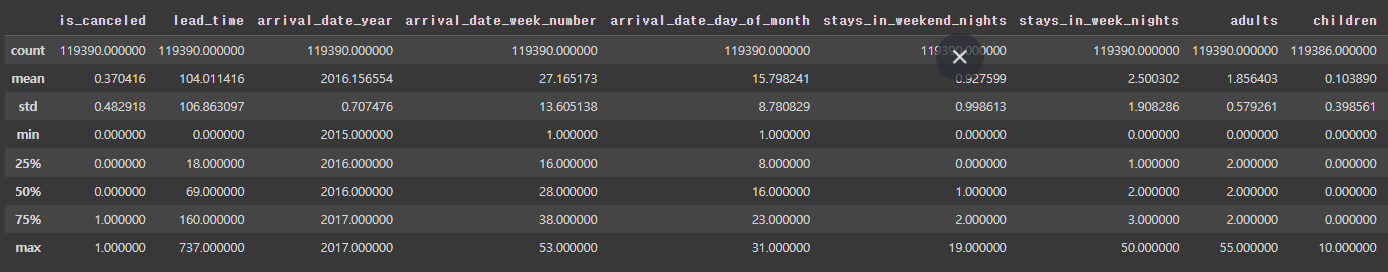
         hotel_df.describe()

         # 아웃라이어 있나 확인

 

 

 

 

• 예약 후 체크인 기간에 따른 취소율

 

 

       sns.displot(hotel_df['lead_time'])

 

  

 

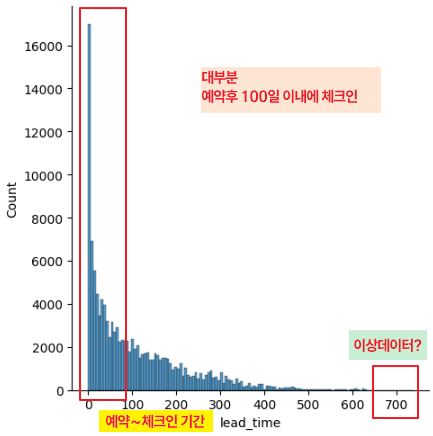• 이상데이터 확인

  

 

        sns.boxplot(y = hotel_df['lead_time'])

 

  

 

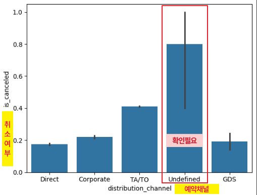
• 예약방법에 따른 취소율

 

 

          sns.barplot(x=hotel_df['distribution_channel'], y=hotel_df['is_canceled'])

          # undefined 데이터 수 확인 필요

 

  

 

 

• 예약채널에 대한 고유 값에 대한 빈도수

  

     

        hotel_df['distribution_channel'].value_counts()

 

  

 

 

 

 

• 호텔에 따른 취소율

  

 

        sns.barplot(x=hotel_df['hotel'], y=hotel_df['is_canceled'])

 

 

 

 

• 년도에 따른 취소율

 

 

        sns.barplot(x=hotel_df['arrival_date_year'], y=hotel_df['is_canceled'])

 

  

 

 

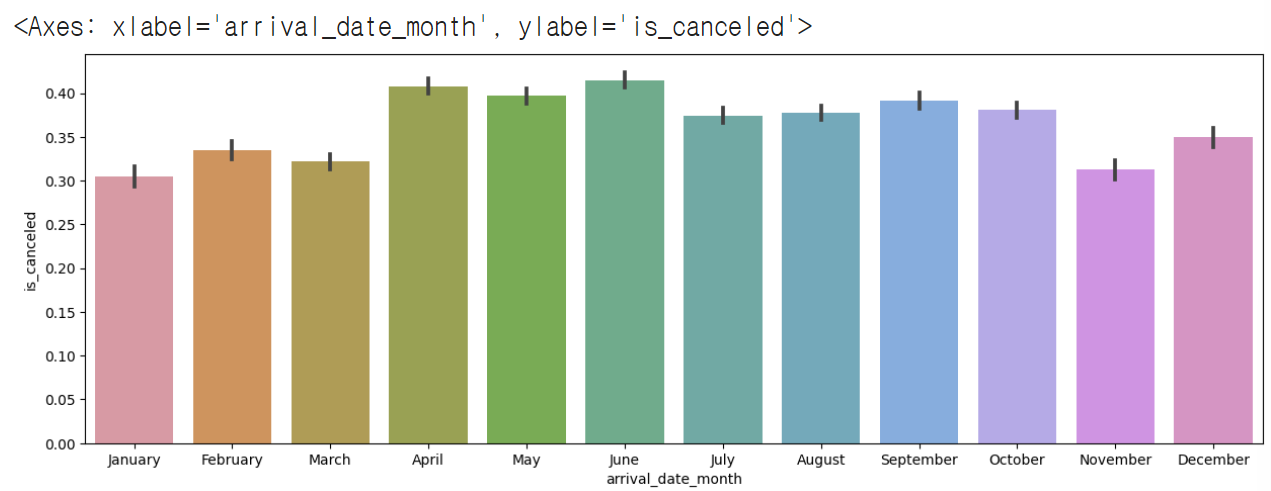
• 월에 따른 취소율

  

 

        plt.figure(figsize=(15,5))

        sns.barplot(x=hotel_df['arrival_date_month'], y=hotel_df['is_canceled'])

 

  

 

• calendar 모듈  사용하기 

 

 

        # 월별로 x축을 정렬하기

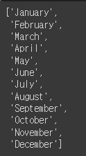
        import calendar

 

        print(calendar.month_name[1])

        print(calendar.month_name[2])

        print(calendar.month_name[3])

  

 

 

• calendar 모듈을 사용하여 월(月)의 이름을 리스트에 저장

  

          months = []

          for i in range(1, 13):

            months.append(calendar.month_name[i])

           

          months

 

 

 

 

• 월별로 x축 정렬하기

 

          # order로 정렬 가능

          plt.figure(figsize=(15,5))

          sns.barplot(x=hotel_df['arrival_date_month'], y=hotel_df['is_canceled'], order=months)

 

 

 

 

• 호텔 방문경험이 취소율에 미치는 영향

       

      sns.barplot(x=hotel_df['is_repeated_guest'], y=hotel_df['is_canceled'])

      # 처음 온 사람이 취소 확률이 더 높다.

  

 

 

• 요금 납부 방식에 따른 취소율

 

 

      sns.barplot(x=hotel_df['deposit_type'], y=hotel_df['is_canceled'])

 

  

 

 

• 요금납부 방식의 고유 값에 대한 빈도수

  

 

      hotel_df['deposit_type'].value_counts()

 

  

 

 

 

• corr() : 열들 간의 상관관계를 계산하는 함수 (피어슨 상관계수)
  # -1 ~ 1까지의 범위를 가지며 0에 가까울수록 두 변수의 상관관계가 없거나 매우 약함
  # -1에 가까울수록 음의 상관관계, 1에 가까울수록 양의 상관관계

  

 

 

        plt.figure(figsize=(15,15))

        sns.heatmap(hotel_df.corr(numeric_only=True), cmap='coolwarm', vmax=1, vmin=-1, annot=True)

        # vmin~vmax 이 사이값으로 정규화 시킴

        # annot=True 네모 박스안에 숫자를 넣기

        # red: 양의 상관관계, blue: 음의 상관관계 -> 색이 진할수록 깊은 관계가 있음

 

 

 

 

•  null인 값 확인

 

 

        hotel_df.isna().mean()

 

 

 

 

• null인 열 삭제

  

 

          hotel_df = hotel_df.dropna()

          hotel_df

  

 

 

 

• 어른이 0인 값

 

 

      hotel_df[hotel_df['adults']==0]

 

  

 

 

• people 파생변수

  

 

        # people 파생변수 만들기

        hotel_df['people'] = hotel_df['adults'] + hotel_df['children'] + hotel_df['babies']

        hotel_df

 

  

 

 

• people이 0인 데이터 이상데이터가 아닐까 추정

 

 

        hotel_df[hotel_df['people']==0]

 

 

 

• people이 0인 경우 삭제

  

 

          hotel_df = hotel_df[hotel_df['people'] != 0]

          hotel_df

  

 

 

• [total_nights] 총 숙박일수 파생변수 만들기

 

 

          hotel_df['total_nights'] = hotel_df['stays_in_week_nights'] + hotel_df['stays_in_weekend_nights']

          hotel_df.head()

 

 

 

 

• [total_nights] 총 숙박일수 0인게 이상
  그런데 데이터가 640개라서 일단 삭제하지 않기

  

 

      hotel_df[hotel_df['total_nights'] == 0]

  

 

 

 

• arrival_date_month 열에 있는 월(month) 정보를 계절(season)로 변환하는 방법

  

          hotel_df['arrival_date_month'].apply(lambda x: 'spring' if x in ['March', 'April', 'May']

                                                                    else 'summer' if x in ['June', 'July', 'August']

                                                                    else 'fall' if x in ['September', 'October',  'November']

                                                                    else 'winter')

 

  

 

 

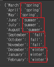
• season 딕셔너리 만들기

 

 

          # arrival_date_month를 참조

 

          # 12, 1, 3: winter # 3, 4, 5: spring  # 6, 7, 8: summer  # 9, 10, 11: fall

 

        season_dic = {'spring': [3,4,5], 'summer': [6,7,8], 'fall': [9,10,11], 'winter':[12,1,2]}

        new_season_dic = {}

        for i in season_dic:

          for j in season_dic[i]:

            new_season_dic[calendar.month_name[j]] = i

        new_season_dic

 

 

 

 

• season 파생변수 생성

  

 

        hotel_df['season'] = hotel_df['arrival_date_month'].map(new_season_dic)

        hotel_df.head()

 

  

 

 

• season 파생변수 생성 확인

 

 

        hotel_df.info()

 

 

 

 

• 예약한 대로 배정이 되었는지가 취소율과 관련이 있을지 확인하기 위해 
  'expected_room_type' 파생변수 생성

  

 

 

        hotel_df['expected_room_type'] = (hotel_df['reserved_room_type'] == hotel_df['assigned_room_type']).astype(int)

        hotel_df.head()

 

 

 

 

 

• 취소율

 

 

        hotel_df['cancel_rate'] = hotel_df['previous_cancellations'] / (hotel_df['previous_cancellations'] + hotel_df['previous_bookings_not_canceled'])

        hotel_df.head()

 

  

 

• [ cancel_rate ] 열의 값이 결측값(NaN)인 행들을 필터링하여 선택

  

     

          hotel_df[hotel_df['cancel_rate'].isna()]

 

 

 

 

• [cancel_rate] 열에서 결측값(즉, NaN)을 -1로 대체

 

          hotel_df['cancel_rate'] = hotel_df['cancel_rate'].fillna(-1)

 

          hotel_df.info()

 

  

 

 

• 데이터 타입을 확인

 

 

        hotel_df['hotel'].dtype # dtype('O') object만 'O'라고 나옴

 

 

        hotel_df['is_canceled'].dtype

 

  

        hotel_df['children'].dtype

 

 

 

 

• object인 열(문자열 열)을 찾아서 obj_list 리스트에 저장

  

 

 

        obj_list = []

        for i in hotel_df.columns:

            if hotel_df[i].dtype == 'O':

                obj_list.append(i)

          obj_list

 

  

 

 

• object 타입 열의 고유한 값의 개수를 출력

 

 

          for i in obj_list:

              print(i, hotel_df[i].nunique())

 

  

 

 

• 문자열 열 중에 고유값이 많은 열삭제

  

 

        hotel_df.drop(['country', 'arrival_date_month'], axis=1, inplace=True)

 

        obj_list.remove('country')

        obj_list.remove('arrival_date_month')

 

 

 

 

• 원핫인코딩

 

      hotel_df = pd.get_dummies(hotel_df, columns=obj_list)

      hotel_df.head()

 

 

 

 

• 데이터 나누기 
  학습용(train)과 테스트용(test) 
  

  

 

          from sklearn.model_selection import train_test_split

          X_train, X_test, y_train, y_test = train_test_split(hotel_df.drop('is_canceled', axis=1), hotel_df['is_canceled'], test_size=0.3, random_state=10)

 

 

 

 

• 데이터 확인

 

 

        X_train.shape , y_train.shape

  

        X_test.shape , y_test.shape

 

  

X 학습 데이터  : 83109개의 샘플(행)과 64개의 특성(열) y 학습 데이터 :  83109 개의 샘플(행) X 테스트 데이터 : 35619개의 샘플(행)과 64개의 특성(열) y 테스트 데이터 : 35619개의 샘플(행)

 

 

2. 앙상블(Ensemble) 모델

-  여러개의 머신러닝 모델을 이용해 최적의 답을 찾아내는 기법을 사용하는 모델

 

보팅(Voting)  * 다른 알고리즘 model을 조합해서 사용  * 모델에 대해 투표로 결과를 도출 배깅(Bagging) * 같은 알고리즘 내에서 다른 sample 조합을 사용 * 샘플 중복 생성을 통해 결과를 도출(K-Fold처럼 데이터 셋 샘플링(조합)을 다르게 하는 듯..) 부스팅(Boosting) * 약간 학습기들을 순차적으로 학습시켜 강력한 학습기를 만듦 * 이전 오차를 보완해가면서 가중치를 부여 * 성능이 매우 우수하지만, 잘못된 레이블이나 아웃라이어에 대해 필요 이상으로 민감할 수 있음 * AdaBoost, Gradient Boosting, XGBoost, LightGBM 스태킹(Stacking * 다양한 개별 모델들으 조합하여 새로운 모델을 생성 * 다양한 모델들을 학습시켜 예측 결과를 얻은 다음 다양한 모델들의 예측

 

 

 

3.  랜덤 포레스트

  

* 머신러닝에서 많이 사용되는 앙상블 기법 중 하나, 결정나무를 기반으로 함 * 학습을 통해 구성해놓은 결정나무로부터 분류결과를 취합하여 결론을 얻는 방식 * 성능은 꽤 우수한 편이나 오버피팅하는 경향이 있음 * 랜덤 포레스트의 트리는 원본 데이터에서 무작위로 선택된 샘플을 기반으로 학습 * 각 트리가 서로 다른 데이터셋으로 학습되어 다양한 트리가 생성되며 모델의 양성이 증가함 * 각각의 트리가 예측한 결과를 기반으로 다수결 또는 평균을 이용하여 최종 예측을 수행함 * 분류와 회귀문제에 모두 사용될 수 있으며 특히 데이터가 많고 복잡한 경우에 매우 효과적인 모델

 

• 학습시키기

  

 

        from sklearn.ensemble import RandomForestClassifier

        rf=RandomForestClassifier()

        rf.fit(X_train, y_train)

 

 

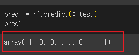
• 모의고사

 

 

        pred1 = rf.predict(X_test)

        pred1

 

 

 

 

• 머신 러닝 모델에서 예측 확률을 계산하여 반환

  

 

      proba1 = rf.predict_proba(X_test)

      proba1

 

 

 

• 첫번째 테스트 데이터에 대한 예측결과

         

      # 첫번째 테스트 데이터에 대한 예측 결과

      proba1[0]

 

 

 

 

• 모든 테스트 데이터에 대한 호텔 예약을 취소할 확률만 출력

 

 

          # 모든 테스트 데이터에 대한 호텔 예약을 취소할 확률만 출력

          proba1[:, 1]

 

 

 

 

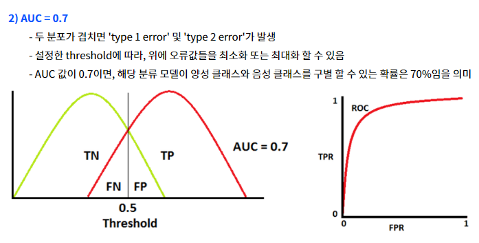
4. 머신러닝/ 딥러닝에서 모델의 성능을 평가하는데 사용하는 측정값

  

 

Accuracy: 올바른 예측의 비율 Precision: 모델에서 수행한 총 긍정 예측 수에 대한 참 긍정 예측의 비율 Recall: 실제 긍정 사례의 총 수에 대한 참 긍정 예측의 비율 F1 Score: 정밀도와 재현율의 조화 평균이며, 정밀도와 재현율 간의 균형을 맞추기 위한 단일 매트릭으로 사용 AUG-ROC Curve : 참양성률과 가양성를 간의 균형을 측정 AUC: ROC 커브와 직선 사이의 면접을 의미  ROC Curve: 이진 분류의 성능을 측정하는 도구, 민감도와 특이도 사이의 관계 참고 사이트: https://bioinformaticsandme.tistory.com/328

 

 

• 머신 러닝 모델의 예측 결과를 평가하기 위해 여러 메트릭과 리포트를 생성

  

 

      from sklearn.metrics import accuracy_score, confusion_matrix, classification_report, roc_auc_score

      accuracy_score(y_test, pred1) # 예측을 한쪽으로 몰아치지는 않았다는걸 알 수 있음

 

      confusion_matrix(y_test, pred1) # 예측을 한쪽으로 몰아치지는 않았다는걸 알 수 있음

 

      print(classification_report(y_test, pred1)) # support는 데이터 갯수

 

 

accuracy_score(y_test, pred1): accuracy_score 함수는 예측된 클래스 레이블 (pred1)과 실제 클래스 레이블 (y_test) 사이의 정확도를 계산합니다. 정확도는 모델이 정확하게 예측한 샘플의 비율을 나타냅니다. 예를 들어, 정확도가 0.85라면 모델이 전체 테스트 데이터에서 85%를 올바르게 예측했다는 것을 의미합니다. confusion_matrix(y_test, pred1): confusion_matrix 함수는 예측된 클래스 레이블 (pred1)과 실제 클래스 레이블 (y_test) 사이의 혼동 행렬(confusion matrix)을 생성합니다. 혼동 행렬은 True Positive, False Positive, True Negative, False Negative의 개수를 보여주어 모델의 분류 성능을 시각적으로 평가하는 데 사용됩니다. 예를 들어, 이 혼동 행렬에서 대각선 요소들이 주 대각선에 가까울수록 모델이 더 정확하게 예측한 것입니다. print(classification_report(y_test, pred1)): classification_report 함수는 정밀도(Precision), 재현율(Recall), F1 점수(F1-Score) 및 각 클래스의 지원 데이터 수(Support)를 포함한 분류 리포트를 출력합니다. Precision은 모델이 positive 클래스로 예측한 것 중에서 실제로 positive인 비율을 나타내며, Recall은 실제 positive 샘플 중에서 모델이 올바르게 예측한 비율입니다. F1-Score는 Precision과 Recall의 조화 평균으로, 모델의 정밀도와 재현율을 종합적으로 평가합니다. Support는 각 클래스의 데이터 개수를 의미합니다.

 

 

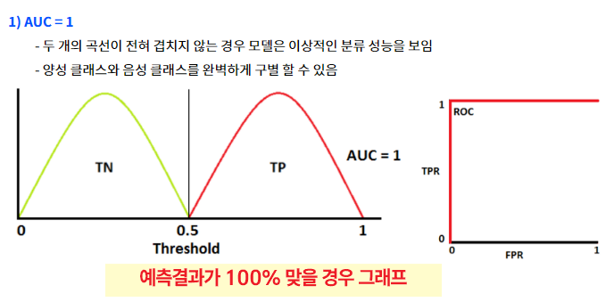
• ROC 곡선 아래 면적을 계산

 

  

        roc_auc_score(y_test, proba1[:, 1])

       # ROC 곡선 아래 면적을 계산하는 함수

 

  

예측결과가 잘 맞다

 

 

• 하이퍼파라미터 수정 (max_depth=30을 적용)

  

 

        # 하이퍼파라미터 수정 (max_depth=30을 적용)

        rf2 = RandomForestClassifier(max_depth=30, random_state=2024)

        rf2.fit(X_train, y_train)

        proba2 = rf2.predict_proba(X_test)

        roc_auc_score(y_test, proba2[:, 1])

        # 하이퍼 파라미터 적용 전: 0.9315576511541386

        # 하이퍼 파라미터 적용(max_depth=30을 적용) 후: 0.9319781899069026

 

        # 하이퍼 파라미터 수정후

        0.9319781899069026 - 0.9315576511541386 = 0.0004205387527640436

 

 

깊이를 30으로 바꾸니 성능이 좋아짐

 

 

• 시각화

 

 

        import matplotlib.pyplot as plt

        from sklearn.metrics._plot.roc_curve import roc_curve

 

        fpr, tpr, thr = roc_curve(y_test, proba2[:, 1])

        print(fpr, tpr, thr)

 

        plt.plot(fpr, tpr, label='ROC Curve')

        plt.plot([0, 1], [0, 1])

        plt.show()

 

 

 

 

• 하이퍼파라미터 수정 

 

 

          # 하이퍼파라미터 추가 수정

          # max_depth=30을 적용

          # min_samples_split=5를 적용

          # n_estimators = 70을 적용

          rf3 = RandomForestClassifier( min_samples_split=5, n_estimators=70, max_depth=30, random_state=2024)

          rf3.fit(X_train, y_train)

          proba3 = rf3.predict_proba(X_test)

          roc_auc_score(y_test, proba3[:, 1])

  

 

          # 하이퍼 파라미터 수정(max_daepth=30을 적용) : 0.9319781899069026

          0.9304821256640659 - 0.9319781899069026 = -0.0014960642428367699 (음수값)

 

 

학습을 덜 하니까 성능이 안좋아짐 (음수값)

 

 

 

 

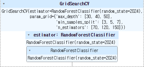
5. 하이퍼 파라미터 최적의 값을 찾는 방법

 * GridSearchCV: 원하는 모든 하이퍼 파라미터를 적용하여 최적의 값을 찾아주는 방법
* RandomizedSearchCV: 원하는 하이퍼 파라미터를 지정하고 n_iter 값을 설정하여 해당 수 만큼 random하게 조합하여 최적의 값을 찾음

 

• 랜덤 포레스트 모델을 사용하여 그리드 서치(Grid Search)를 수행하여 최적의 하이퍼파라미터를 찾는 과정

  

 

          from sklearn.model_selection import GridSearchCV

 

        # 하이퍼파라미터 그리드 정의

          params = {

              'max_depth': [30, 40, 50],

              'min_samples_split': [3, 5, 7],

              'n_estimators': [70, 120, 150]

          }

 

        # 랜덤 포레스트 모델 초기화

          rf4 = RandomForestClassifier(random_state=2024)

 

        # 그리드 서치 객체 생성

          grid_df = GridSearchCV(rf4, params) # cv: 데이터 교차검증

 

        # 그리드 서치 수행

          grid_df.fit(X_train, y_train)

 

 

 

 

 

• params 중에서 최고의 하이퍼파라미터 조건 출력

 

 

        grid_df.best_params_

        # params 중에서 최고의 하이퍼파라미터 조건을 보여줌

 

  

 

 

• grid_df.cv_results_는 GridSearchCV 객체에서 제공하는 속성
  그리드 서치 과정에서 각 하이퍼파라미터 조합에 대한 세부 정보를 포함하는 딕셔너리

  

 

        grid_df.cv_results_

 

 

 

 

• 랜덤 포레스트 모델을 사용하여 랜덤 서치(Randomized Search)를 수행하여
  최적의 하이퍼파라미터를 찾는 과정

 

 

        rf5 = RandomForestClassifier(random_state=2024)

 

        rand_df = RandomizedSearchCV(rf5, params, n_iter=4, random_state=2024)

 

        rand_df.fit(X_train, y_train)

 

 

 

 

• params 중에서 최고의 하이퍼파라미터 조건

  

        rand_df.best_params_

 

 

 

• 그리드 서치 과정에서 각 하이퍼파라미터 조합에 대한 세부 정보를 포함하는 딕셔너리 출력

 

      

        rand_df.cv_results_

 

  

 

 

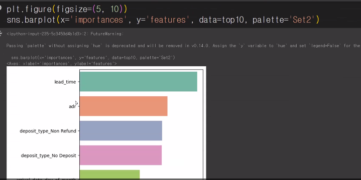
6. 피처 중요도(Feature Importances)

   

 

• 랜덤 포레스트 분류기(RandomForestClassifier)를 사용하여 모델을 학습하고 예측하는 과정

  

 

        rf6 = RandomForestClassifier(random_state=2024, max_depth=40, min_samples_split=3, n_estimators = 150)

        rf6.fit(X_train, y_train)

        proba6 = rf6.predict_proba(X_test)

        roc_auc_score(y_test, proba2[:, 1])

  

 

0.9316574459006468

 

 

• proba6는 rf6.predict_proba(X_test)의 결과
  테스트 데이터 X_test에 대한 예측된 클래스별 확률을 담고 있는 배열

 

 

      proba6

 

  

 

 

• rf6.feature_importances_는 랜덤 포레스트 모델rf6에서 각 특성(feature)의 중요도(importance)를 나타내는 속성
  주어진 값인 1.27823051e-01은 특성의 중요도를 나타내는 하나의 숫자

  

 

        rf6.feature_importances_

 

        1.27823051e-01

  

 

 

 

• X_train.columns: 학습 데이터 X_train의 열(특성) 이름들을 나타내는 속성
• rf6.feature_importances_: 랜덤 포레스트 모델 rf6에서 계산된 각 특성의 중요도 값

  

 

        feat_imp = pd.DataFrame({

            'features': X_train.columns,

            'importances': rf6.feature_importances_

        })

        feat_imp

  

 

 

• feat_imp 에서 중요도(importance) 값에 따라 내림차순으로 정렬한 후 상위 10개의 행

 

 

        top10 = feat_imp.sort_values('importances', ascending=False).head(10)

        top10

 

  

 

 

• 상위 10개의 중요한 특성(feature)을 시각화

  

 

        plt.figure(figsize=(5,10))

        sns.barplot(x='importances', y='features', data=top10, palette='Set2')