⏺ 나이브 베이즈 분류기
나이브 베이즈 분류기
|
나이브 베이즈 분류기는 확률론과 베이즈 정리를 기반으로 하는
|
나이브 베이즈 분류기
|
|
나이브 베이즈 분류기
|
나이브 베이즈 분류기 모델 |
모델의 특성 |
|
| 1 |
Gaussian Naive Bayes |
연속형 데이터를 다루며, 각 feature가 정규 분포를 따른다고 가정합니다. [예] 성적, 키, 몸무게 등 연속적인 값이 있는 데이터에 적합합니다. |
| 2 |
Multinomial Naive Bayes |
이산형 데이터를 다루며, feature가 다항 분포를 따른다고 가정합니다. [예] 텍스트 분류(단어 빈도), 문서 분류 등에서 사용됩니다. |
| 3 |
Bernoulli Naive Bayes |
이진형 데이터를 다루며, 각 feature가 0 또는 1의 값을 가질 때 적합합니다. [예] 텍스트 분류(단어 존재 여부), 스팸 메일 분류 등에서 사용됩니다. |
| 4 |
Complement Naive Bayes |
Multinomial Naive Bayes의 변형으로, 불균형한 데이터셋에 대해 더 나은 성능을 보입니다. [예] 텍스트 분류에서 클래스 불균형 문제를 다룰 때 유용합니다. |
| 5 |
Categorical Naive Bayes |
범주형 데이터를 다루며, feature가 유한한 수의 카테고리 값을 가질 때 적합합니다. [예] 설문 조사 데이터, 범주형 속성 데이터를 처리할 때 사용됩니다. |
✔ HR 데이터
승진 여부를 예측하기 위한 데이터 전처리 과정
- 데이터 전처리 전
 |
데이터 전처리 과정 |
|
필요없는 열 삭제 |
|
null인 행 삭제 |
|
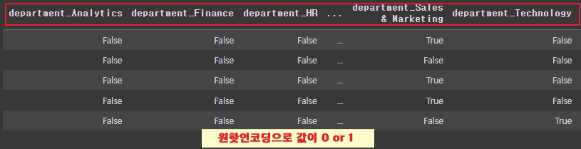
원핫인코딩
|
|
 |
|
스케일링
|
|
 |
|
- 데이터 전처리 완료
 |
- 데이터를 학습용(train)과 테스트용(test)으로 분할
|
X_train, X_test, y_train, y_test = train_test_split(hr_df1.drop('is_promoted', axis=1), hr_df1['is_promoted'], test_size=0.2, random_state=999)
|
|
- 학습용(train)과 테스트용(test) 데이터
|
X_train.shape, X_test.shape
# 결과 ((38928, 23), (9732, 23))
X_train : 38928개의 샘플 / 샘플당 23개의 특성(열)
y_train : 38928개의 레이블(타겟) |
|
y_train.shape, y_test.shape
# 결과 ((38928,), (9732,))
X_test : 9732개의 샘플 / 샘플당 23개의 특성(열)
y_test : 9732개의 레이블(타겟)
|
1. 분석 ver1
나비스 베이스 5가지 모델 비교
나이브 베이즈 분류기 모델 |
모델의 특성 |
|
| 1 |
Gaussian Naive Bayes |
연속형 데이터를 다루며, 각 feature가 정규 분포를 따른다고 가정합니다. [예] 성적, 키, 몸무게 등 연속적인 값이 있는 데이터에 적합합니다. |
| 2 |
Multinomial Naive Bayes |
이산형 데이터를 다루며, feature가 다항 분포를 따른다고 가정합니다. [예] 텍스트 분류(단어 빈도), 문서 분류 등에서 사용됩니다. |
| 3 |
Bernoulli Naive Bayes |
이진형 데이터를 다루며, 각 feature가 0 또는 1의 값을 가질 때 적합합니다. [예] 텍스트 분류(단어 존재 여부), 스팸 메일 분류 등에서 사용됩니다. |
| 4 |
Complement Naive Bayes |
Multinomial Naive Bayes의 변형으로, 불균형한 데이터셋에 대해 더 나은 성능을 보입니다. [예] 텍스트 분류에서 클래스 불균형 문제를 다룰 때 유용합니다. |
| 5 |
Categorical Naive Bayes |
범주형 데이터를 다루며, feature가 유한한 수의 카테고리 값을 가질 때 적합합니다. [예] 설문 조사 데이터, 범주형 속성 데이터를 처리할 때 사용됩니다. |
평가지표 |
계산방법 |
||
| 1 |
accuracy_score |
정확도 | 전체 예측 중 맞춘 비율 -----> 전체 직원 중에서 승진 여부를 정확히 맞춘 비율 |
| 2 |
Precision |
정밀도 | 모델이 양성이라고 예측한 것 중에서 실제 양성의 비율 TP / (TP + FP) -----> 승진한다고 예측한 직원 중에서 실제로 승진한 직원의 비율 |
| 3 |
Recall |
재현율 | 실제 양성 중에서 모델이 양성으로 정확히 예측한 비율 TP / (TP + FN) ------> 실제로 승진한 직원 중에서 모델이 정확히 승진 예측한 비율 |
| 4 |
F1 Score |
정밀도와 재현율의 조화 평균 |
정밀도와 재현율 간의 균형 : F1 스코어가 높을수록 정밀도와 재현율의 균형이 잘 맞는다는 것을 의미 |
- 나이브 베이즈 분류기 모델을 생성
|
from sklearn.naive_bayes import GaussianNB, MultinomialNB, BernoulliNB, ComplementNB, CategoricalNB gnb = GaussianNB() # 가우시안
mnb = MultinomialNB() # 다항분포
bnb = BernoulliNB() # 베르누이
cpb = ComplementNB() # 컴플리먼트
cgb = CategoricalNB() # 카테고리
|
- Gaussian Naive Bayes (GaussianNB) 모델을 사용하여 학습
테스트 데이터에 대해 예측한 결과의 여러 평가 지표를 출력
|
gnb.fit(X_train, y_train)
pred = gnb.predict(X_test)
print('GaussianNB')
print('accuracy_score',accuracy_score(y_test, pred))
print('precision_score',precision_score(y_test, pred))
print('recall_score',recall_score(y_test, pred))
print('f1_score',f1_score(y_test, pred))
|
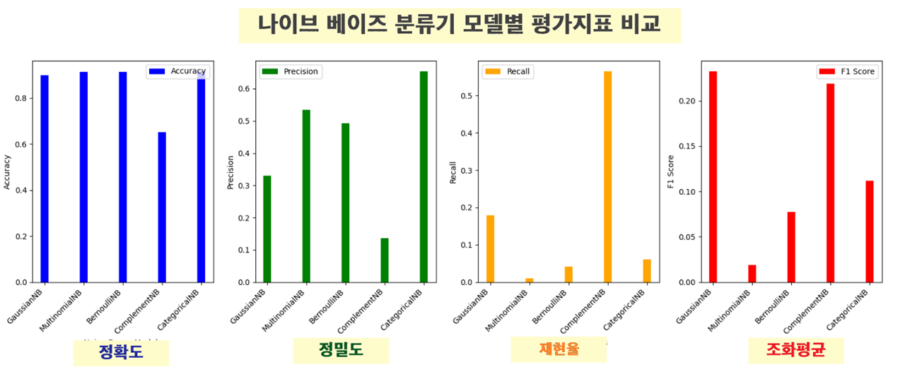
| GaussianNB accuracy_score 0.8981709823263461 precision_score 0.3303964757709251 recall_score 0.17921146953405018 f1_score 0.23237800154918667 |
- Multinomial Naive Bayes (MultinomialNB) 모델을 사용하여 학습하고
테스트 데이터에 대해 예측한 결과의 여러 평가 지표를 출력
|
mnb.fit(X_train, y_train)
pred = mnb.predict(X_test)
print('MultinomialNB')
print('accuracy_score',accuracy_score(y_test, pred))
print('precision_score',precision_score(y_test, pred))
print('recall_score',recall_score(y_test, pred))
print('f1_score',f1_score(y_test, pred))
|
| MultinomialNB accuracy_score 0.9140978216193999 precision_score 0.5333333333333333 recall_score 0.009557945041816009 f1_score 0.018779342723004692 |
- Bernoulli Naive Bayes (BernoulliNB) 모델을 사용하여 학습하고
테스트 데이터에 대해 예측한 결과의 여러 평가 지표를 출력
|
bnb.fit(X_train, y_train)
pred = bnb.predict(X_test)
print('BernoulliNB')
print('accuracy_score',accuracy_score(y_test, pred))
print('precision_score',precision_score(y_test, pred))
print('recall_score',recall_score(y_test, pred))
print('f1_score',f1_score(y_test, pred))
|
| BernoulliNB accuracy_score 0.9138923140156185 precision_score 0.49295774647887325 recall_score 0.04181600955794504 f1_score 0.07709251101321586 |
- Complement Naive Bayes (ComplementNB) 모델을 사용하여 학습하고
테스트 데이터에 대해 예측한 결과의 여러 평가 지표를 출력
|
cpb.fit(X_train, y_train)
pred = cpb.predict(X_test)
print('ComplementNB')
print('accuracy_score',accuracy_score(y_test, pred))
print('precision_score',precision_score(y_test, pred))
print('recall_score',recall_score(y_test, pred))
print('f1_score',f1_score(y_test, pred))
|
| ComplementNB accuracy_score 0.6525893958076449 precision_score 0.1355300859598854 recall_score 0.5651135005973715 f1_score 0.21862722440489948 |
- Categorical Naive Bayes (CategoricalNB) 모델을 사용하여 학습하고
테스트 데이터에 대해 예측한 결과의 여러 평가 지표를 출력
|
cgb.fit(X_train, y_train)
pred = cgb.predict(X_test)
print('CategoricalNB')
print('accuracy_score',accuracy_score(y_test, pred))
print('precision_score',precision_score(y_test, pred))
print('precision_score',recall_score(y_test, pred))
print('f1_score',f1_score(y_test, pred))
|
| CategoricalNB accuracy_score 0.9164611590628853 precision_score 0.6538461538461539 recall_score 0.06093189964157706 f1_score 0.11147540983606558 |
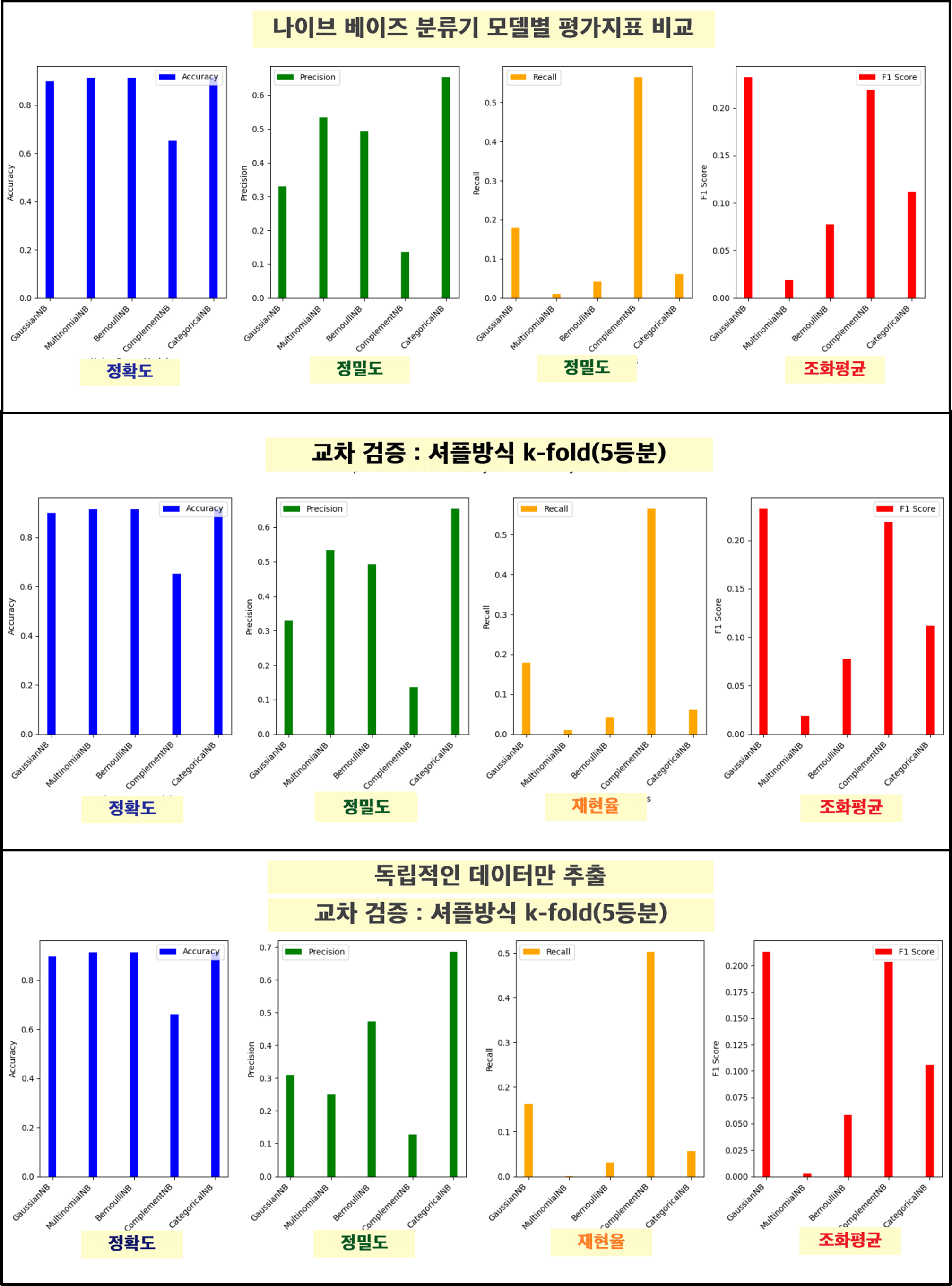
- 다섯 가지 Naive Bayes 모델 그래프 생성
|
import numpy as np
import matplotlib.pyplot as plt
from sklearn.metrics import accuracy_score, precision_score, recall_score, f1_score
from sklearn.model_selection import train_test_split
from sklearn.naive_bayes import GaussianNB, MultinomialNB, BernoulliNB, ComplementNB, CategoricalNB
def compare_naive_bayes_models(X_train, X_test, y_train, y_test):
# 다섯 가지 Naive Bayes 모델 초기화
gnb = GaussianNB()
mnb = MultinomialNB()
bnb = BernoulliNB()
cpb = ComplementNB()
cgb = CategoricalNB()
models = [gnb, mnb, bnb, cpb, cgb]
model_names = ['GaussianNB', 'MultinomialNB', 'BernoulliNB', 'ComplementNB', 'CategoricalNB']
# 성능 지표 계산을 위한 빈 리스트 초기화
accuracy_scores = []
precision_scores = []
recall_scores = []
f1_scores = []
# 각 모델별로 성능 지표 계산
for model in models:
model.fit(X_train, y_train)
y_pred = model.predict(X_test)
accuracy_scores.append(accuracy_score(y_test, y_pred))
precision_scores.append(precision_score(y_test, y_pred))
recall_scores.append(recall_score(y_test, y_pred))
f1_scores.append(f1_score(y_test, y_pred))
# 그래프 생성
x = np.arange(len(model_names))
width = 0.2
fig, axs = plt.subplots(1, 4, figsize=(16, 6))
fig.suptitle('Comparison of Naive Bayes Models by Metrics', fontsize=16)
# Accuracy
axs[0].bar(x, accuracy_scores, width, label='Accuracy', color='blue')
axs[0].set_xlabel('Naive Bayes Models')
axs[0].set_ylabel('Accuracy')
axs[0].set_xticks(x)
axs[0].set_xticklabels(model_names, rotation=45, ha='right')
axs[0].legend()
# Precision
axs[1].bar(x, precision_scores, width, label='Precision', color='green')
axs[1].set_xlabel('Naive Bayes Models')
axs[1].set_ylabel('Precision')
axs[1].set_xticks(x)
axs[1].set_xticklabels(model_names, rotation=45, ha='right')
axs[1].legend()
# Recall
axs[2].bar(x, recall_scores, width, label='Recall', color='orange')
axs[2].set_xlabel('Naive Bayes Models')
axs[2].set_ylabel('Recall')
axs[2].set_xticks(x)
axs[2].set_xticklabels(model_names, rotation=45, ha='right')
axs[2].legend()
# F1 Score
axs[3].bar(x, f1_scores, width, label='F1 Score', color='red')
axs[3].set_xlabel('Naive Bayes Models')
axs[3].set_ylabel('F1 Score')
axs[3].set_xticks(x)
axs[3].set_xticklabels(model_names, rotation=45, ha='right')
axs[3].legend()
plt.tight_layout()
plt.subplots_adjust(top=0.88)
plt.show()
# 예시 데이터 준비
X_train, X_test, y_train, y_test = train_test_split(hr_df1.drop('is_promoted', axis=1), hr_df1['is_promoted'], test_size=0.2, random_state=999)
# 함수 호출
compare_naive_bayes_models(X_train, X_test, y_train, y_test)
|
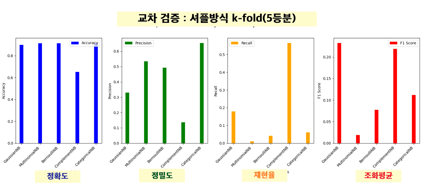
2. 분석 ver2
교차 검증 : 셔플방식 k-fold(5등분)
- 교차 검증
KFold를 사용하여 데이터셋을 여러 개의 부분 집합(folds)으로 나누어 모델을 학습시키고 평가
|
kf = KFold(n_splits=5,random_state=10,shuffle=True
|
|
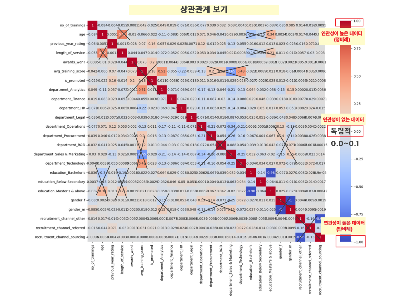
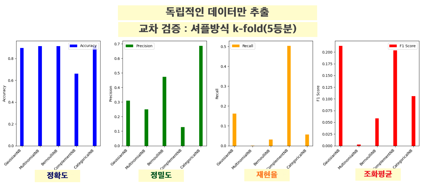
3. 분석 ver3
교차 검증 : 셔플방식 k-fold(5등분)+ 독립적인 데이터만 추출
나이브 베이즈 분류기는 각 feature(특징)가 독립적이라고 가정하기 때문에
서로 값에 영향을 받지 않는 데이터만 추출해서 정확도 높여보기 !
- 상관관계 보기
|
import seaborn as sns
import matplotlib.pyplot as plt
correlation_matrix = hr_df1.corr()
# 상관관계 행렬 히트맵 시각화
plt.figure(figsize=(16, 12))
sns.heatmap(correlation_matrix, annot=True, cmap='coolwarm')
plt.show()
|
 |
- 상관계수 낮은 데이터만 출력
|
correlation_matrix = hr_df1.corr()
# 상관관계 행렬 히트맵 시각화
plt.figure(figsize=(16, 12))
sns.heatmap(correlation_matrix, annot=True, cmap='coolwarm')
plt.show()
|
 |
- 추가적인 열 삭제
[ recruitment_channel_other ]
채용방식에서 기타방식은 여러가지가 합쳐진거라 묶어놓은 개념이라 필요없을거같아서 제거
[ education_Master's & above ]
학력에서 석사이상은 평이한 분석을 위해 인원이 더 많은 학사쪽을 남기기로 택
[ avg_training_score ]
전년도 고과점수는 엮인 칼럼이 많아 여러가지 칼럼들과 상관계수가 높게 나타남
[ age ] [ gender_f ] [ gender_m ]
나이와 성별은 요즘 시대상 반영하여 근속년수 및 성과가 더 중요하다 생각해서 제거
|
hr_df1.drop(['recruitment_channel_other',"education_Master's & above",'avg_training_score','age','gender_f','gender_m'], axis=1, inplace=True)
|
더보기
| 나이브 베이즈 모델은 조건부 독립성을 가정하여 각각의 특성이 서로 독립적이라고 가정합니다. 이 가정 하에 나이브 베이즈 모델은 특성 간의 상관관계를 무시하고 계산합니다. 따라서, 이론적으로 특성들 간의 상관관계가 낮거나 없는 데이터에서 더 잘 작동할 것으로 기대할 수 있습니다. 하지만, 이는 항상 정확도가 더 높게 나온다는 것을 보장하지 않습니다. 그 이유는 다음과 같습니다: 1. 현실 데이터의 복잡성
2. 특성 선택의 중요성
3. 모델의 적합성
|
결론 : 나이브 베이스 모델 중 어떤 모델이 적합할까?

HR 데이터를 분석하기에 적절한 모델?
|
Gaussian Naive Bayes는 연속형 데이터를 잘 처리하며, 계산이 효율적이고 해석이 용이합니다.
Complement Naive Bayes는 불균형 데이터셋에 더 적합하며, 다항 분포를 따르는 데이터에서 더 나은 성능을 발휘할 수 있습니다.
|

- 가우시안 나이브 베이즈

- 컴플리먼트 나이브 베이즈

|
'AI > 머신러닝' 카테고리의 다른 글
| 15. 연관 규칙 학습 | Apriori , Eclat (0) | 2024.10.07 |
|---|---|
| 14. 계층적 군집화(HC) | 고객층 분석 (0) | 2024.10.07 |
| 12. K-평균 군집화 (KMeans) | Marketing (0) | 2024.06.17 |
| 11. 다양한 모델 성능비교 | Air Quality UCI (0) | 2024.06.17 |
| 10. lightGBM | Credit (0) | 2024.06.13 |


